Know whether your data arrived intact — and exactly what didn’t
Every integrity system answers the same question — did this data change? The difference is what they say next. A hash tells you yes or no, nothing else. A Merkle tree can tell you which record changed. Closure tells you which record, how much the value drifted, and whether the sequence was altered or rearranged — a distinction that separates a corruption from a replay attack, and one that has never existed in an integrity primitive before. This additional layer runs on top of the hash you are already computing; the overhead is +5%.
Two tools implement this. The CLI handles file-to-file comparison and live
monitoring of data streams. The bind() / prism
functions handle zero-knowledge verification: two parties confirm they hold
identical data by exchanging 16 bytes, the raw records staying on each side,
the exchange mathematically unforgeable.
What each method actually gives you
| Capability | SHA-256 | Hash Chain | Merkle | Closure |
|---|---|---|---|---|
| Detects any corruption | ✓ | ✓ | ✓ | ✓ |
| Pinpoints the exact record | — | ✓ (slow) | ✓ | ✓ |
| Measures how much it drifted (σ) | — | — | — | ✓ |
| Distinguishes reordering from corruption | — | — | — | ✓ |
| Verify without sharing the raw data | — | — | — | ✓ |
| Recovers the original records | — | — | — | ✓ |
Single-fault localization at scale — 1,000,000 records
| Method | Time to locate | Checks needed | vs Closure | What it reports |
|---|---|---|---|---|
| Closure | 6.5 μs | 20 | — | “record #750,000 drifted by 1.47” |
| Merkle | 13.1 μs | 21 | 2× slower | “record #750,000 differs” |
| Hash Chain | 60.4 ms | 750,001 | 9,245× slower | “something changed” |
| SHA-256 | — | — | — | “something changed” |
Multi-fault detection — 100,000 records
| Faults | Merkle tree | Closure | Speedup |
|---|---|---|---|
| 1 | 368 ms | 362 ms | 1× |
| 5 | 1.85 s | 396 ms | 4.7× |
| 10 | 3.68 s | 383 ms | 9.6× |
| 25 | 9.39 s | 426 ms | 22× |
| 50 | 18.6 s | 384 ms | 48× |
A Merkle tree must rebuild itself after every fault it finds, so the work grows with each new corruption it encounters. Closure walks both sequences once and classifies all faults in that single pass — the time stays flat regardless of how many problems exist. At 50 faults the gap reaches 48×, and it keeps widening from there.
pip install closure-sdk ·
pip install closure-cli ·
GitHub
Storage with integrity built in
Closure DNA is a database you query with standard SQL. As it stores data, it continuously maintains a geometric fingerprint of everything it holds, so when you ask whether your data is intact, the answer comes back in microseconds without scanning any records. Any change to the data — deliberate or accidental — shows up immediately.
Named snapshots work the way git commits do: capture the current state, name it, restore to it exactly whenever you need to. Resonance search finds records that are geometrically similar to a query — which users have tastes closest to this one, which products sit near this one in the catalog, which past events most resemble what is happening now. Two separate installations can compare a single derived value to confirm they hold identical copies of a table, each keeping its records private.
Benchmark against SQLite — 1,000,000 records
SQLite has indexes on all filtered columns. Closure DNA wins on almost every axis.
| Operation | Closure DNA | SQLite | Ratio | Winner |
|---|---|---|---|---|
| Insert | 786.6 ms | 934.8 ms | 1.2× | Closure DNA |
| Get ×1000 | 669 μs | 4.60 ms | 6.9× | Closure DNA |
| Filter city=X (indexed) | 11.9 ms | 81.0 ms | 6.8× | Closure DNA |
| Filter age>50 (indexed) | 20.2 ms | 176.8 ms | 8.8× | Closure DNA |
| city=X AND age>50 | 61.7 ms | 94.6 ms | 1.5× | Closure DNA |
| AVG(score) | 14.6 ms | 53.3 ms | 3.6× | Closure DNA |
| Sort by age | 73.0 ms | 385.0 ms | 5.3× | Closure DNA |
| Update 1 row | 73.9 μs | 164.4 μs | 2.2× | Closure DNA |
| Delete 1 row | 34.4 μs | 84.8 μs | 2.5× | Closure DNA |
| Integrity check | 11.7 μs | 1.05 s | 89,885× | Closure DNA |
| Resonance search | 836.8 ms | N/A | — | Exclusive |
| Table identity check | 13.9 μs | N/A | — | Exclusive |
| Cold start (reopen) | 376.8 μs | 78.1 μs | 4.8× | SQLite |
The tradeoff worth knowing: on 100,000 records, Closure DNA uses 26.5 MB on disk versus 6.1 MB for SQLite. The raw column data is 4.7 MB — comparable to SQLite — but each column carries a geometric sidecar that enables the fast queries, integrity checks, and resonance search. Those sidecars add up to 20.2 MB, and they are fully rebuildable from the data: delete them and they regenerate. The cold-start time reflects the same trade — slightly slower to open, meaningfully faster once running.
pip install closure-dna ·
GitHub
Computation without parameters
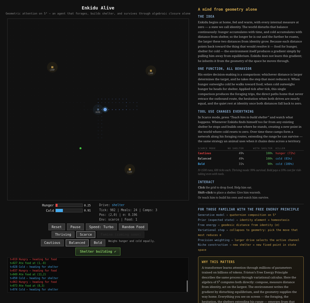
Enkidu is a simulated agent navigating a hostile world: foraging for food, building shelter, staying alive. Every decision comes from a single question — what need is pulling him furthest from balance right now, and what action brings him closest to rest? The same geometry that stores and verifies data also makes that measurement, and the agent acts on whatever the answer is. There is no trained model, because the geometry is already the answer.
Everything you see in the demo — the foraging routes, the hesitation when two drives are equally urgent, the way his territory expands when resources get scarce — emerges from that one operation applied repeatedly to a world that refuses to leave him alone.
The torus knot animating the panel above is lifted directly from Enkidu’s own visualization — the same code, the same geometry, running here as it runs inside the agent.
Why this matters beyond the demo
The behavioral neuroscience community has spent decades building a formal account of how living systems make decisions. The answer it keeps arriving at is the same operation: measure the gap between where you are and where you should be, act on what is most urgent. Enkidu runs that principle directly in arithmetic, and the correspondence to the dominant theory of biological intelligence is exact.
Memory, verification, and execution share one representation — database and compute are the same layer. This is the direction of the work.